Neural Network Notation - From Arrows to Weight Matrices

The Launch Log Comes First

A rocket team keeps a small launch log.

Before every launch attempt, Mission Control records a few clues and makes one call:

GO or HOLD?

Launch ID

Wind (mph)

Fuel (%)

Launch

L001

8

92

GO

L002

22

35

HOLD

L003

12

81

GO

L004

28

41

HOLD

Deep learning notation starts here.

Not with symbols.

---

What the Launch Log Has

Mission Control keeps a small launch log.

Each row is one launch attempt.

Each column records one thing about that attempt.

The table has only four columns:

• Launch ID is just the row name. It identifies the attempt, but it is not a launch clue.
• Wind records the wind speed before launch.
• Fuel records how much fuel is ready.
• Launch records the final call: GO or HOLD.

The model will look at Wind and Fuel.

The model learns the final call: GO or HOLD.

---

From Brain Cells to Rocket Brains

A biological neuron receives many signals.

If the combined signal is strong enough, it activates and sends a new signal forward.

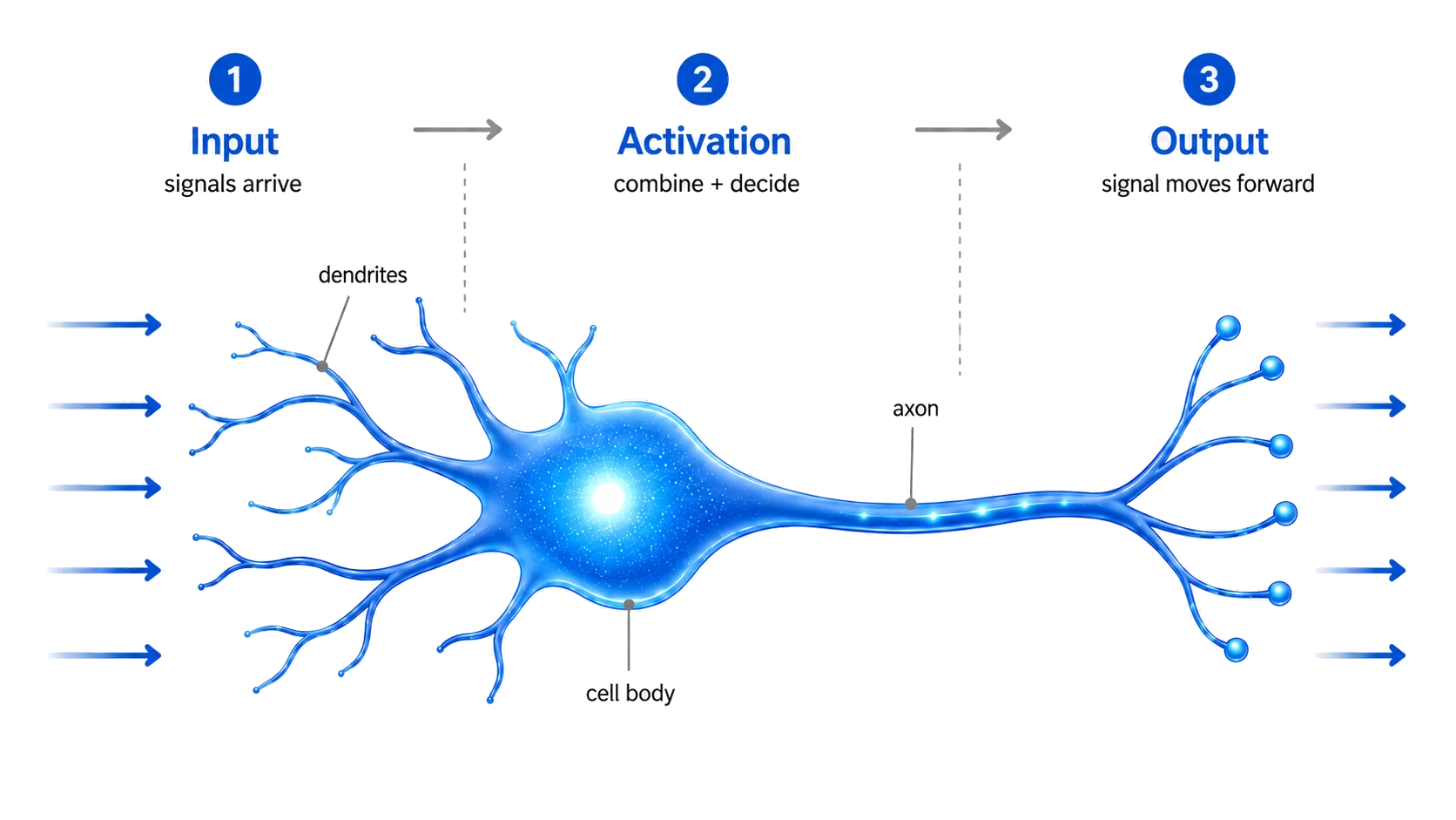
Artificial neurons borrow that flow:

inputs come in → activation happens → output goes out

In our rocket story, the inputs are simple: Wind and fuel.

The clues move through the network until it makes the final call: GO or HOLD.

Control Wind and Fuel to help the rocket launch.

If the final Launch value reaches 60% or higher, Mission Control says GO.

If it stays below 60%, the rocket stays on the pad.

---

Reading the Network Picture

In the network picture, Wind and Fuel are input values.

They are the clues entering the network.

They are not neurons.

The two middle circles are neurons.

Both neurons receive the same input values:

Wind.
Fuel.

But they do not have to listen to them the same way.

Each neuron gives Wind and Fuel its own level of trust.

Then each one sends a signal forward.

Those two signals become the inputs for the final neuron.

The final neuron combines them one more time.

That final result becomes the network’s call:

GO or HOLD.

So this tiny network has three artificial neurons:

Two hidden neurons + one output neuron

---

Zooming Into One Neuron

The network picture shows several circles.

Let’s zoom into Activation 1, one neuron in the middle of the network.

Input: $X$

It receives two inputs:

$$x_1 = \text{Wind}$$ $$x_2 = \text{Fuel}$$

Here, x simply means input.

So $x_1$ is the first input, and $x_2$ is the second input.

Weights: $W$

But Activation 1 does not trust both inputs equally. It asks:

• How much should I listen to Wind?
• How much should I listen to Fuel?

Those “how much should I listen?” numbers are called weights.

$$w_1 = \text{influence of Wind}$$ $$w_2 = \text{influence of Fuel}$$

For Activation 1, the neuron gives more influence to Fuel and less influence to Wind:

$$w_1 = 0.35 \text{ for Wind} \quad w_2 = 0.65 \text{ for Fuel}$$

In plain English:

Fuel carries more influence here, but Wind still matters.

Net Input: $Z$

Now the neuron combines the inputs and weights into one score.

That score is called the net input.

We denote it by $z$:

$$z = w_1x_1 + w_2x_2$$

For Activation 1, that becomes:

$$z = 0.35x_1 + 0.65x_2$$

It is the neuron’s total faith after weighing both clues: Wind and Fuel.

Threshold: $\theta$

But $z$ is just a number, not GO or HOLD yet.

To turn that number into a decision, the neuron compares it to a threshold.

We denote that threshold by $\theta$.

If $z$ reaches or crosses $\theta$, the neuron says GO.

If $z$ stays below $\theta$, the neuron says HOLD.

Earlier, the simulation used 60% as the threshold for launch.

$$\theta = 60$$

So the rule becomes:

$$\sigma(z) = \begin{cases} 1 & \text{if } z \ge \theta \\ 0 & \text{otherwise} \end{cases}$$

That symbol $\sigma$ is the activation function.

Activation Function: $\sigma$

Activation function converts the score $z$ into a clean output:

$$1 = \text{GO}$$ $$0 = \text{HOLD}$$

This is called a step function because it starts at 0 and, once the score crosses the threshold, jumps to 1.

Because the jump has a size of 1, this version is also called a unit step function.

Drag z across the graph and watch what happens when z reaches θ = 60.

Bias: $b$

There is one more small trick.

So far, the neuron compares the score $z$ to a threshold:

$$z \ge \theta$$

In our rocket example:

$$\theta = 60$$

That means:

$$z \ge 60$$

But real neural networks usually do not carry the threshold around separately.

They shift the threshold to zero using a mathematical trick:

$$z - \theta \ge 0$$

Now the new decision rule is simpler:

$$\text{fire if the new score is } \ge 0$$

The threshold line is now zero.

That hidden shift behaves like a bias term.

So the threshold is folded into the net input as $b$:

$$z = w_1x_1 + w_2x_2 + b$$

Think of bias as the launch system’s starting adjustment before it judges Wind and Fuel.

The question is no longer:

Is the bias positive or negative?

The better question is:

Did bias move the score closer to the launch line or farther away?

Notice in the example above, the dotted bias line sits at:

$$b = 12$$

The dotted line shows the bias push, not the final score.

The final score is still the green $z$ dot.

That places bias on the launch side of the zero line.

So this bias makes the network more lenient toward launch.

For example, suppose the weighted clues produce:

$$w_1x_1 + w_2x_2 = -18$$

By itself, the neuron says HOLD.

With bias 12:

$$z = -18 + 12 = -6$$

Closer, but still below zero.

Still HOLD.

With bias 20:

$$z = -18 + 20 = 2$$

Now the score crosses zero.

The neuron says GO.

Bias does not change Wind or Fuel.

Bias changes how much help the score gets before the final check:

$$\sigma(z) = \begin{cases} 1 & \text{if } z \ge 0 \\ 0 & \text{otherwise} \end{cases}$$

The neuron still asks:

Did the score cross the line?

Bias just changes how close the score starts to that line.

🧭 Notation Checkpoint

Before we zoom out to matrix notation, here is the notation we just met:

Symbol	Reads as	Meaning in our rocket story
$x$	input	One clue entering the neuron
$x_1$	first input	Wind
$x_2$	second input	Fuel
$w$	weight	How much the neuron listens to an input
$w_1$	first weight	Influence of Wind
$w_2$	second weight	Influence of Fuel
$z$	net input	The weighted score before the final decision
$\theta$	threshold	The launch line the score must cross
$\sigma(z)$	activation function	The rule that turns the score into output
$b$	bias	The starting adjustment that moves the score closer to or farther from the launch line

The whole neuron can now be read as:

$$z = w_1x_1 + w_2x_2 + b$$

Then the activation function asks:

$$\sigma(z) = \begin{cases} 1 & \text{if } z \ge 0 \\ 0 & \text{otherwise} \end{cases}$$

---

Writing the Same Neuron in Matrix Notation

So far, we wrote the neuron one piece at a time:

$$z = w_1x_1 + w_2x_2 + b$$

That is clear, but it gets tiring fast.

If a rocket launch has two clues, this is fine.

If it has twenty clues, the formula becomes a long grocery receipt.

Matrix notation is the shortcut.

It lets us pack the inputs and weights into neat columns.

One Launch Attempt as a Vector

For one launch attempt, the neuron watches two clues:

$$x_1 = \text{Wind} \qquad x_2 = \text{Fuel}$$

Matrix notation stacks them into one input vector:

$$x = \begin{bmatrix} \text{Wind} \\ \text{Fuel} \end{bmatrix} = \begin{bmatrix} x_1 \\ x_2 \end{bmatrix}$$

The weights can be stacked the same way:

$$w = \begin{bmatrix} \text{how much Wind matters} \\ \text{how much Fuel matters} \end{bmatrix} = \begin{bmatrix} w_1 \\ w_2 \end{bmatrix}$$

So one launch attempt gives the neuron two vectors:

$$x = \begin{bmatrix} x_1 \\ x_2 \end{bmatrix} \qquad w = \begin{bmatrix} w_1 \\ w_2 \end{bmatrix}$$

The inputs say what the neuron sees.

The weights say how much the neuron listens to each input.

In books, you may see the same column vector written sideways like this:

$$x = [x_1 ; x_2]$$

That compact notation means the same thing as:

$$x = \begin{bmatrix} x_1 \\ x_2 \end{bmatrix}$$

Books write it sideways to save vertical space, but the semicolon tells you it is still a column vector.

Dot Product: The Short Version of the Score

The neuron still needs the score:

$$z = w_1x_1 + w_2x_2 + b$$

The weighted part is:

$$w_1x_1 + w_2x_2$$

We already stacked the inputs and weights as vectors:

$$x = \begin{bmatrix} x_1 \\ x_2 \end{bmatrix} \qquad w = \begin{bmatrix} w_1 \\ w_2 \end{bmatrix}$$

To multiply them, we transpose the weight vector:

$$w^T = \begin{bmatrix} w_1 & w_2 \end{bmatrix}$$

Now the weighted part can be written as:

$$w^T x = \begin{bmatrix} w_1 & w_2 \end{bmatrix} \begin{bmatrix} x_1 \\ x_2 \end{bmatrix} = w_1x_1 + w_2x_2$$

This row-times-column operation is called a dot product.

Now we add bias to the score:

$$z = w^T x + b$$

In this one-neuron version:

• $w^T x$ gives one weighted score
• $b$ gives one bias adjustment
• $z$ becomes one final score

Same neuron.

Cleaner notation.

---

From One Launch Attempt to a Matrix

So far, the neuron scored one launch attempt:

$$z = w^T x + b$$

That is useful, but real training data is not one row.

It is a table.

Single row input: $x$

One launch attempt has two input features:

$$x_1 = \text{Wind} \qquad x_2 = \text{Fuel}$$

For one launch attempt, we can write those two values as one row:

$$\begin{bmatrix} x_1^{(1)} & x_2^{(1)} \end{bmatrix}$$

Here is the small notation trick:

$$\large x_{\text{C} \vphantom{\rule{0pt}{2.0ex}} }^{\rule{0pt}{3.5ex}(\text{R})} \quad \begin{array}{l} \leftarrow \small \text{launch attempt} \\ \leftarrow \small \text{feature \#} \end{array}$$

RC = Row, Column.

This is the same RC idea from the earlier Machine Learning Notation guide.

Machine Learning Notation Review the RC memory hook. →

Now read the two symbols in that row:

$$\large \begin{array}{ccc} x_1^{(1)} \begin{array}{l} \leftarrow \small \text{launch 1} \\ \leftarrow \small \text{feature 1} \end{array} & \; & x_2^{(1)} \begin{array}{l} \leftarrow \small \text{launch 1} \\ \leftarrow \small \text{feature 2} \end{array} \end{array}$$

Both values come from launch attempt 1.

But they sit in different feature columns.

That is one launch attempt.

Matrix input: $X$

Now add a second launch attempt.

The table grows downward:

$$\begin{array}{rccl} & \small \text{feature 1} & \small \text{feature 2} & \\ & \downarrow & \downarrow & \\ X = \Bigg[ \!\!\! & \begin{array}{c} x_1^{(1)} \\[1.5ex] x_1^{(2)} \end{array} & \begin{array}{c} x_2^{(1)} \\[1.5ex] x_2^{(2)} \end{array} & \!\!\! \Bigg] \!\! \begin{array}{l} \leftarrow \small \text{launch 1} \\[1.5ex] \leftarrow \small \text{launch 2} \end{array} \end{array}$$

This is the first big jump.

Lowercase $x$ was one launch attempt.

Capital $X$ is a collection of launch attempts.

So with two launch attempts and two features, $X$ has shape:

$$2 \times 2$$

Scoring the matrix with $w$

The number of weights is tied to the number of features, not the number of launch attempts.

We could have one launch attempt, ten launch attempts, or a full logbook.

But if each launch attempt has two features, the neuron needs two weights:

$$\large w = \begin{bmatrix} w_1 \\ w_2 \end{bmatrix} \quad \begin{array}{l} \leftarrow \small \text{weight for feature 1} \\ \leftarrow \small \text{weight for feature 2} \end{array}$$

For one launch attempt, we used:

$$z = w^T x + b$$

That gave one weighted score.

But now we are no longer scoring one launch attempt.

We are scoring the whole launch logbook.

So the notation changes:

$$w^T x \quad \longrightarrow \quad Xw$$

$w^T x$ scores one launch attempt.

$Xw$ scores every launch attempt in $X$.

The dimensions explain why:

$$w^T x = (1 \times 2)(2 \times 1) = 1 \times 1$$

That gives one weighted score for one launch attempt.

But the launch logbook has many rows:

$$Xw = (\# \times 2)(2 \times 1) = \# \times 1$$

That gives one weighted score for each launch attempt.

Same idea.

Different organization.

For the two-row launch logbook:

$$\underbrace{ \begin{bmatrix} x_1^{(1)} & x_2^{(1)} \\[1.5ex] x_1^{(2)} & x_2^{(2)} \end{bmatrix} }_{X} \; \underbrace{ \begin{bmatrix} w_1 \vphantom{x_1^{(1)}} \\[1.5ex] w_2 \vphantom{x_1^{(2)}} \end{bmatrix} }_{w} = \begin{bmatrix} w_1x_1^{(1)} + w_2x_2^{(1)} \\[1.5ex] w_1x_1^{(2)} + w_2x_2^{(2)} \end{bmatrix}$$

Same weights.

Two launch attempts. Two weighted scores.

Adding bias

Now add bias.

The bias is one adjustment value:

$$b$$

But $Xw$ returns a column of weighted scores:

$$Xw = \begin{bmatrix} \text{score}^{(1)} \\[1.5ex] \text{score}^{(2)} \end{bmatrix}$$

So when we write:

$$z = Xw + b$$

we mean:

$$z = \begin{bmatrix} \text{score}^{(1)} + b \\[1.5ex] \text{score}^{(2)} + b \end{bmatrix}$$

The same bias is applied to each launch attempt’s weighted score.

So $z$ becomes a column of final scores:

$$z = \begin{bmatrix} z^{(1)} \\[1.5ex] z^{(2)} \end{bmatrix}$$

One final score per launch attempt.

General shape

If the launch logbook has $n$ launch attempts and $m$ input features, then $X$ has shape:

$$n \times m$$

The weight vector needs one weight per feature, so $w$ has shape:

$$m \times 1$$

Now the shape of $Xw$ is:

$$Xw = (n \times m)(m \times 1) = n \times 1$$

So $Xw$ gives $n$ scores — one per launch attempt.

$$Xw = \begin{bmatrix} \text{score}^{(1)} \\ \text{score}^{(2)} \\ \vdots \\ \text{score}^{(n)} \end{bmatrix}$$

Then bias shifts the score column:

$$z = Xw + b$$

The bias $b$ is added to each score:

$$z = \begin{bmatrix} \text{score}^{(1)} + b \\ \text{score}^{(2)} + b \\ \vdots \\ \text{score}^{(n)} + b \end{bmatrix}$$

So $z$ becomes the final score column.

In code, you usually do not manually build that repeated bias column.

You pass $b$ once, and the library applies it across the score column.

lowercase $x$ is one launch attempt.
capital $X$ is the launch logbook.
$Xw + b$ scores the whole logbook.

---

From scores to decisions

Now $z$ is a column of scores.

But raw scores are not the goal — HOLD or GO is.

The activation function $\sigma$ converts scores into decisions:

$$\hat{y} = \sigma(z)$$

The hat matters.

$\hat{y}$ means the model’s prediction.

It is not the actual ground-truth label $y$.

So in our rocket story:

• $y$ is what really happened: GO or HOLD
• $\hat{y}$ is what the neuron predicted: GO or HOLD

A step function is one kind of activation function:

$$\sigma(z) = \begin{cases} 1 & \text{if } z \ge 0 \\ 0 & \text{otherwise} \end{cases}$$

So each score becomes a decision:

$$\hat{y} = \begin{bmatrix} \hat{y}^{(1)} \\ \hat{y}^{(2)} \\ \vdots \\ \hat{y}^{(n)} \end{bmatrix}$$

One decision per launch attempt.

Insight: $z$ is the score.
$\hat{y}$ is the decision.

🧭 Matrix Notation Checkpoint

Here is the capital notation we just met:

Symbol	Shape	Meaning
$X$	$n \times m$	Full launch logbook
$w$	$m \times 1$	One weight per feature
$Xw$	$n \times 1$	One weighted score per launch attempt
$b$	repeated across $n$ scores	Bias adjustment
$z$	$n \times 1$	Final score column
$\sigma(z)$	$n \times 1$	Activation applied to each score
$\hat{y}$	$n \times 1$	Prediction column

Memory hook:

$X$ is the launch logbook. $Xw + b$ scores it. $\sigma(z)$ turns scores into predictions.

---

Mission Control Briefing

Capital X: The Full Logbook

Mission Control opens the binder of launch attempts. That full table is X.

Capital X: The Full Logbook. Mission Control opens the binder of launch attempts. That full table is X.

Quiz

86% of people love quizzes after learning. Are you one of them?

★

Question 1 of 12 🏆 0 / 120 ⚡ Attempt 1 of 2

Question text

Next →

From One Neuron to the Network Map

Next: Read the Whole Network Now that one neuron makes sense, zoom out and learn how layers, arrows, weights, and matrix shapes fit together. →