How Logits and Sigmoid Power Logistic Regression

When a Score Is Not the Answer

Have you ever found yourself wondering:

• The Fan: Your team has home advantage, and the opponent’s best player is injured. What are the chances your team wins?
• The Student: You attended every lecture, studied for ten hours, and slept well. What are the chances you pass?
• The Runner: You followed the training plan and recovered well. What are the chances you finish the marathon?
• The Producer: Early reviews are strong, and ticket sales are rising. What are the chances the movie becomes a hit?
• The Traveler: The weather is clear, but the incoming plane is already delayed. What are the chances your flight arrives on time?

Behind each question, many pieces of evidence can be combined into a raw score:

• Team advantage score: +3.3
• Exam readiness score: +1.6
• Marathon readiness score: +2.4
• Movie success score: +4.1
• On-time arrival score: -1.2

These scores tell us which way the evidence is leaning. Positive scores lean toward the outcome. Negative scores lean away from it.

But a score like 3.8 is not the answer anyone actually wants.

We want an answer like: There is an 80% chance.

So we need to translate between two spaces:

1. An unrestricted space of raw scores
2. A probability space between 0 and 1

That translation is where logits and the sigmoid function enter the story.

---

Reverse Engineering the Translation

Return to the sports fan.

A predictive model combines the evidence:

• Home advantage adds $+2.4$
• The opponent’s injury adds $+1.7$
• Other evidence pulls the score down by $-0.8$

After combining everything, the model produces an unrestricted score:

$$2.4 + 1.7 - 0.8 = +3.3$$

In practice, we want to turn that raw score of $+3.3$ into the probability of our team winning:

$$\text{Raw score} \rightarrow \text{Probability}$$

But to figure out that translation, we have to build the math in the opposite direction.
We will stretch a probability into a raw score, and then reverse that transformation.

Here is the two-part journey:

Part 1: Stretch Probability into a Logit

• 1A — Probability to Odds: Stretch $0$–$1$ across the positive number line.
• 1B — Odds to Logits: Extend that positive scale across the full range from $-\infty$ to $+\infty$.

Part 2: Reverse the Journey

• 2 — Logits to Probability: Use the sigmoid to fold the unrestricted scale back into $0$–$1$.

Let’s start by stretching probability into odds.

---

1A. Probability to Odds

Our first step is to stretch probability from the bounded $0$–$1$ range into the positive number line.

Probability tells us how often something succeeds out of all possible outcomes.

Odds compare success directly with failure:

$$\text{Odds} = \frac{\text{Success}}{\text{Failure}} = \frac{P}{1-P}$$

Suppose your team has an 80% chance of winning:

• Chance of winning (success): $0.8$
• Chance of losing (failure): $1 - 0.8 = 0.2$

The odds are:

$$\text{Odds} = \frac{0.8}{0.2} = 4$$

The odds are 4 to 1.

For every four wins, we expect one loss.

Try clicking different points on the curve.

At $50\%$, the odds are $1:1$.

One win for every loss. The outcome is perfectly balanced.

Now click a point below $50\%$.

At $25\%$, the odds are about $0.33$, or $1:3$.

For every win, there are three losses. Failure is more likely.

Now click a point above $50\%$.

At $80\%$, the odds are $4:1$.

For every loss, there are four wins.

As you move closer to $100\%$, the curve rises sharply. A probability that is still squeezed below $1$ can become odds of $4$, $9$, $19$, and beyond.

Notice what happened to the range:

• Probability can only live between $0$ and $1$
• Odds can range from $0$ to $+\infty$

Odds have stretched the small probability range across the entire positive side of the number line.

But they still cannot become negative. To reach from $-\infty$ to $+\infty$, we need one more transformation.

---

1B. Odds to Logits

Our next step is to extend odds across the entire number line.

Because odds are always positive, we take their logarithm to create both negative and positive values:

$$\text{Logit} = \log(\text{Odds}) = \log\left(\frac{P}{1-P}\right)$$

The word logit was coined by statistician Joseph Berkson in 1944.

It was created as a companion to probit, another way of transforming probability.

The name comes from:

log unit → logit

A logit is simply the logarithm of the odds.

Probability 0.50

Odds 1.00

Logit 0.00

Click a point below $50\%$, then one above it.

Watch what happens to the logit:

• Below $50\%$, it moves into negative numbers
• At $50\%$, it lands on $0$
• Above $50\%$, it moves into positive numbers

That gives logit space a natural center: $0$ means success and failure are perfectly balanced.

Now compare the ranges:

• Probability: $0$ to $1$
• Odds: $0$ to $+\infty$
• Logits: $-\infty$ to $+\infty$

Odds opened the positive side of the number line. Logits opened the whole line.

The score can now move anywhere from $-\infty$ to $+\infty$.

But the original questions were asking for a probability:

• What are the chances my team wins?
• What are the chances I pass?
• What are the chances my flight arrives on time?

So how do we turn this open-ended score into a number between $0$ and $1$?

---

2. Logits to Probability

We need a function that can take any value on the number line and gently bend it back into probability space.

That curve is called the logistic sigmoid, or simply the sigmoid function:

$$P = \sigma(z) = \frac{1}{1+e^{-z}}$$

Here, $z$ is the logit.

Drag across the curve and watch how the same score is translated into probability.

Try these three regions:

• Move far left: large negative logits become probabilities close to $0$
• Stop at the center: $z=0$ becomes $P=0.5$
• Move far right: large positive logits become probabilities close to $1$

Notice how the curve never crosses below $0$ or above $1$. It bends the entire logit range from $-\infty$ to $+\infty$ into probability space.

“Sigmoid” is the broader name for a family of S-shaped curves.

The curve used here is the logistic curve, also called the logistic sigmoid. It traces back to Belgian mathematician Pierre-François Verhulst, who used it in the 1830s to model population growth.

Other sigmoid curves include the Gompertz curve, hyperbolic tangent, and error function.

The two transformations now work in opposite directions:

$$P \xrightarrow{\text{logit}} z \xrightarrow{\text{sigmoid}} P$$

Logit opens probability onto the whole number line. Sigmoid folds it back between $0$ and $1$.

---

Back to the Sports Fan

We started with the model’s raw score:

$$\text{Logit} = 3.3$$

To understand what that score meant, we first built the mathematics in reverse:

$$\text{Probability} \rightarrow \text{Odds} \rightarrow \text{Logit}$$

Now we reverse that path with the sigmoid:

$$P = \frac{1}{1+e^{-3.3}} \approx 0.964$$

So the model’s raw score of $3.3$ becomes:

A $96.4\%$ probability that our team wins.

The model worked on the unrestricted logit line. The sigmoid translated its final score into the answer the fan actually wanted.

---

The Big Picture: Logistic Regression

Why did we build an unrestricted number line?

Because models are good at combining evidence with a linear equation:

$$z = \boldsymbol{w}^\top \boldsymbol{x} + b$$

The linear equation produces an unrestricted raw score, making it unsuitable as a probability on its own.

Logistic regression keeps that unrestricted score for the calculation, then uses the sigmoid to translate it into probability.

Logistic regression handles this in two stages:

1. Build an unrestricted linear score from the evidence.
2. Pass that score through the sigmoid to turn it into probability.

1. Build the Logit

First, logistic regression combines the evidence into one unrestricted linear score.

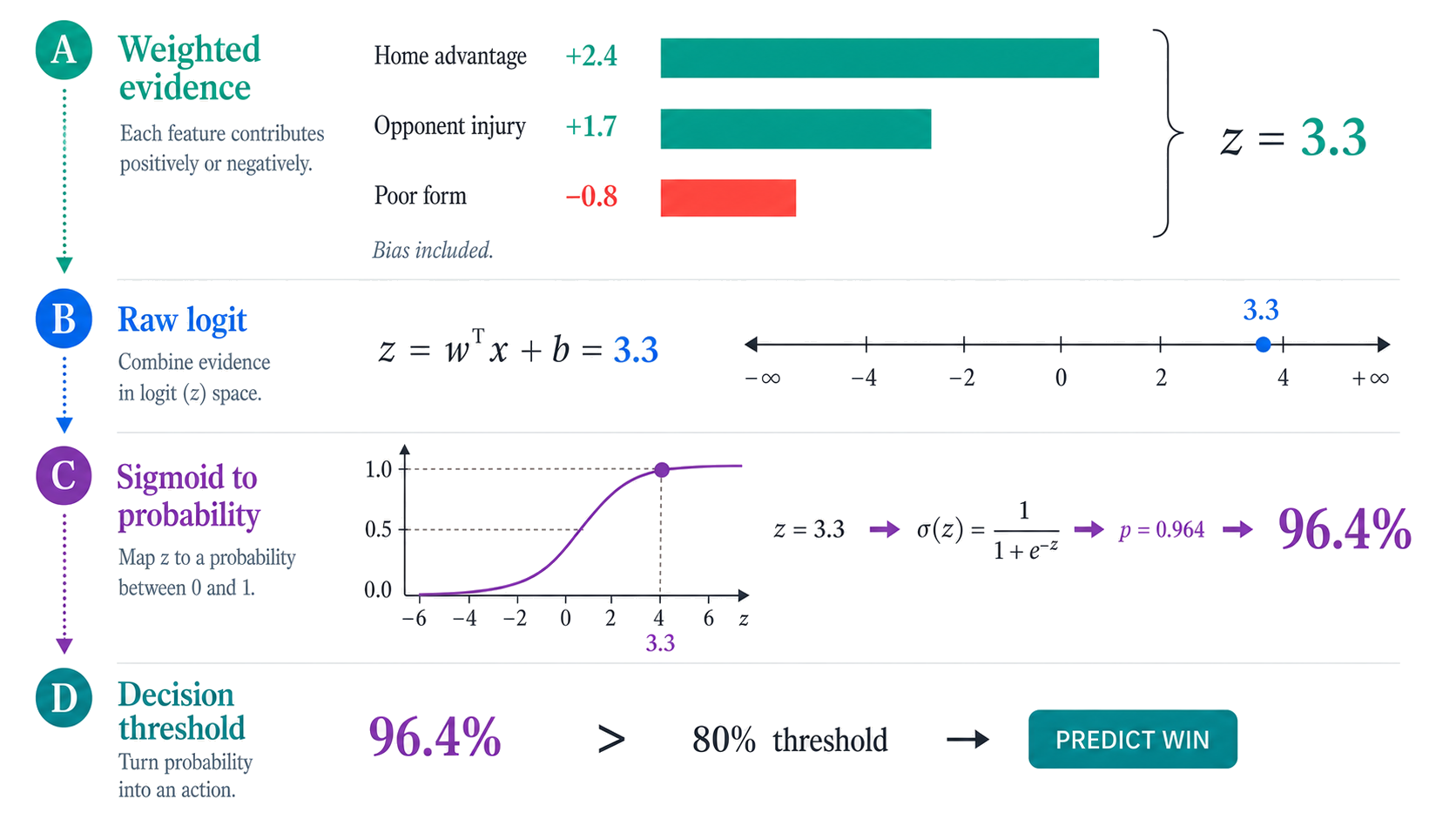
The model combines its input features into a weighted sum:

$$z = \boldsymbol{w}^\top \boldsymbol{x} + b$$

For our sports fan:

$$z = 2.4 + 1.7 - 0.8 = 3.3$$

Logistic regression treats this unrestricted score as the log-odds:

$$\log\left(\frac{p}{1-p}\right) = \boldsymbol{w}^\top \boldsymbol{x} + b$$

This works because logits can move freely from $-\infty$ to $+\infty$, just like a linear equation.

Why can we treat the linear score as log-odds?

Because they are mathematically compatible. A linear equation can produce any value from $-\infty$ to $+\infty$, and log-odds live on that same unrestricted scale.

So logistic regression makes this core modeling assumption:

$$\text{Linear score} = \text{Log-odds}$$

That gives the model open space to combine evidence while preserving a reversible path back to probability.

2. Translate the Logit into Probability

Next, the sigmoid folds that unrestricted score into the $0$–$1$ probability range.

The logit is the link between probability and the linear score.

To return to probability, we reverse that link with the logistic sigmoid:

$$p = \sigma(z) = \frac{1}{1+e^{-z}}$$

For our raw score of $3.3$:

$$p = \frac{1}{1+e^{-3.3}} \approx 0.964$$

So logistic regression estimates:

A $96.4\%$ probability that our team wins.

The full journey is:

$$\text{Features} \rightarrow \text{Linear score} \rightarrow \text{Logit} \rightarrow \text{Sigmoid} \rightarrow \text{Probability}$$

Turning Probability into a Decision

Finally, a threshold converts the probability into a class or action.

The model produces a probability, not a class label.

A decision rule can then convert that probability into an action:

$$p \ge 0.5 \rightarrow \text{Win}$$ $$p < 0.5 \rightarrow \text{Loss}$$

The threshold does not have to be $0.5$. It depends on the cost of making each kind of mistake.

Why Is It Called Logistic Regression?

Logistic comes from the logistic function—the S-shaped curve used to convert logits into probabilities.

Regression comes from modeling the log-odds with a linear equation:

$$\log\left(\frac{p}{1-p}\right) = \boldsymbol{w}^\top \boldsymbol{x} + b$$

It is commonly used for classification, but the model itself first estimates a probability.

Logistic regression draws a straight line in logit space, then bends it into probability space.

Why Is It Still a Linear Model?

The sigmoid is curved, so why is logistic regression considered a linear model?

Because the score underneath is built as an additive linear combination:

$$z = w_1x_1 + w_2x_2 + \cdots + w_nx_n + b$$

Each feature contributes its own weighted amount, and those contributions are added together.

The sigmoid only translates that linear score into probability. It does not change the linear structure underneath.

The engine is linear. The sigmoid is the translator.

---

Logistic Regression in One Picture

---

Concept Check

Odds

Four wins for every one loss. Odds compare success directly with failure and stretch from $0$ to $+\infty$.

Odds. Four wins for every one loss. Odds compare success directly with failure and stretch from $0$ to $+\infty$.

Quiz

86% of people love quizzes after learning. Are you one of them?

★

Question 1 of 12 🏆 0 / 120 ⚡ Attempt 1 of 2

Question text

Next →